MATH 221 × CE 122
When does a tumour stop growing?
The architects of the simulation.
This computational audit of Subramanian et al. (2025) was engineered collaboratively by five students spanning Electrical and Computer Engineering at Ashesi University.





A mathematical audit of proliferation.
This project investigates the dynamics of breast tumour growth using the Gompertz differential equation, grounded in experimental murine data from Subramanian et al. (2025). We replicate the primary model, perform a rigorous numerical error analysis comparing explicit Euler and Runge-Kutta (RK4) methods, and extend the framework by introducing a linear proportional treatment term.
Our central result is that under a proportional kill term the treated model collapses exactly onto a Gompertz model with a reduced ceiling $K' = Ke^{-d/a}$, and that the substitution $u = \ln V$ turns the whole system into a first-order linear ODE driven by the dose. The tumour becomes a first-order plant; the dose becomes its input.
Engineering relevance: This is a control-systems problem at its core. The tumour is a dynamic system; treatment is the control input; the carrying capacity is a stability boundary. The same differential-equation tools that model spring-mass-dampers and RLC circuits — equilibrium analysis, numerical integration, error convergence — are exactly what let an engineer predict tumour trajectories, locate the dose that holds a tumour at stasis, and show why no finite constant dose drives the system to zero. Biology becomes a plant to be controlled.
The geometry of survival.
Cancer is fundamentally a failure of spatial mathematics. Healthy cells possess contact inhibition; they stop dividing when resources run out or space is constrained. Malignant cells ignore these signals. Early attempts to model tumours relied on simple exponential growth, which inaccurately assumes infinite biological resources.
The Gompertz equation provides a vital correction. It introduces a carrying capacity, mathematically forcing the growth rate to decay as the tumour mass expands and its necrotic core is starved of oxygen and nutrients. Accurate forecasting of this curve is crucial for timing therapeutic interventions.
The experimental data underpinning this model comes from a xenograft study: human LM2-4LUC⁺ triple-negative breast carcinoma cells implanted into 6–8 week-old female mice. Tumour volume was measured directly with calipers and computed as $V = \frac{\pi}{6} w^2 L$, where $L$ and $w$ are the largest and smallest tumour diameters. This gives us real volumetric growth data from a living biological system — the ground truth our model must reproduce.
A single equation, fitted to life.
Early tumour models assumed exponential growth — cells dividing without limit. This fails biologically: as a tumour expands, its necrotic core is starved of oxygen and nutrients, and physical space constraints slow division. The Gompertz model corrects this by introducing a carrying capacity that forces the growth rate to decay as volume increases. It has been the most widely applied model in oncology precisely because it captures this sigmoid deceleration accurately.
Subramanian et al. (2025) fit the Gompertz differential equation to caliper-derived volumetric measurements from murine breast tumours. The model is expressed as:
where each term carries a precise biological meaning:
| Symbol | Meaning | Value (Subject 1) |
|---|---|---|
| $V(t)$ | Tumour volume at time $t$ | mm³ |
| $t$ | Time since first measurement | days (window: 22 – 31.6) |
| $a$ | Intrinsic growth rate — controls how fast the tumour grows when small | 0.3 day⁻¹ |
| $K$ | Carrying capacity — the maximum sustainable tumour volume | 1200 mm³ |
| $V_0$ | Initial volume at the start of the observation window | 619 mm³ |
| $\ln(K/V)$ | The biological brake — approaches zero as $V \to K$, halting growth | dimensionless |
The parameters $a = 0.3$ day⁻¹ and $K = 1200$ mm³ were determined by Subramanian et al. by fitting the model to caliper measurements from Subject ID=1 using the TRBDF2 ODE solver. The initial condition $V_0 = 619$ mm³ is not a direct measurement — it is an interpolated value. Section VIII sets out exactly where it comes from and how much it actually matters.
Integrating the ODE exactly yields the analytical solution — no numerical approximation required:
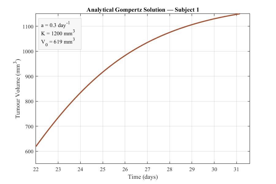
This closed-form expression lets us evaluate $V$ at any time $t$ directly. As $t \to \infty$, the exponential term vanishes and $V(t) \to K$, confirming that the tumour asymptotically approaches its carrying capacity regardless of initial size.
Gompertz Growth — Analytical Solution V(t)
Recreating the original results.
To validate our implementation, we replicate Figure 2 from Subramanian et al. (2025) for murine Subject ID=1. Our MATLAB implementation uses identical parameters: $a = 0.3$ day$^{-1}$, $K = 1200$ mm$^3$, $V_0 = 619$ mm$^3$.
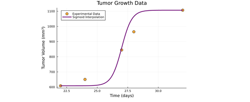
Figure 1 — Sigmoid Interpolation of Raw Data. The paper preprocesses five sparse caliper measurements using a sigmoid interpolation to produce a smooth growth curve. We replicate this below.
Original · Subramanian et al. (2025) Fig. 1
Our Replication · MATLAB Implementation
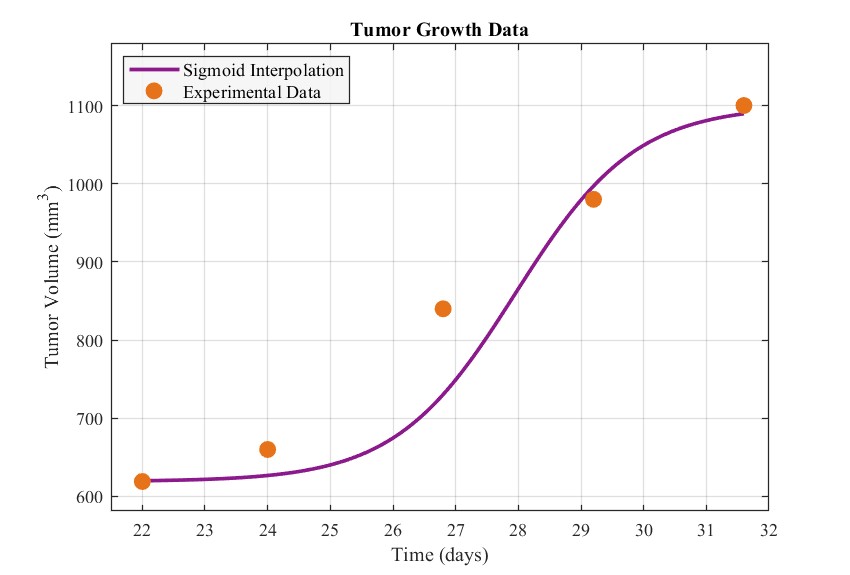
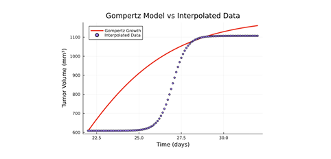
Figure 2 — Gompertz Model vs Interpolated Data. The Gompertz ODE is solved analytically and compared against the sigmoid-interpolated data. The model captures the general growth trend but overestimates volume during the mid-phase — a key finding we return to when we assess the limits of the model.
Original · Subramanian et al. (2025) Fig. 2
Our Replication · MATLAB Implementation
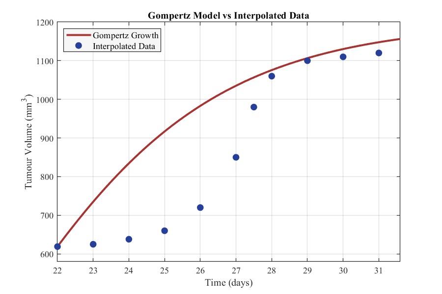
Validation: Our Figure 1 replication confirms the sigmoid interpolation correctly captures the S-shaped growth curve from five sparse measurements. In Figure 2, the Gompertz curve rises from $V_0 = 619$ mm$^3$ and saturates toward $K = 1200$ mm$^3$, matching the published trajectory. The visible overestimation in the mid-phase (days 25–28) is consistent with the paper's own finding — a genuine structural limitation of the Gompertz form, which we record in Section XII rather than paper over.
A note on small visual differences: The paper's plots are not based on raw data — only five caliper measurements exist per subject. The authors fit a sigmoid interpolation through those sparse points and plot the Gompertz model against that interpolated curve. Our replication uses the identical five points and identical Gompertz parameters, but minor differences in the fitted sigmoid (its steepness and midpoint) shift the interpolated curve slightly. The mathematically significant behaviour — the mid-phase overestimation — is reproduced exactly, confirming our model is correct.
Approximating the analytical truth.
The Euler Method
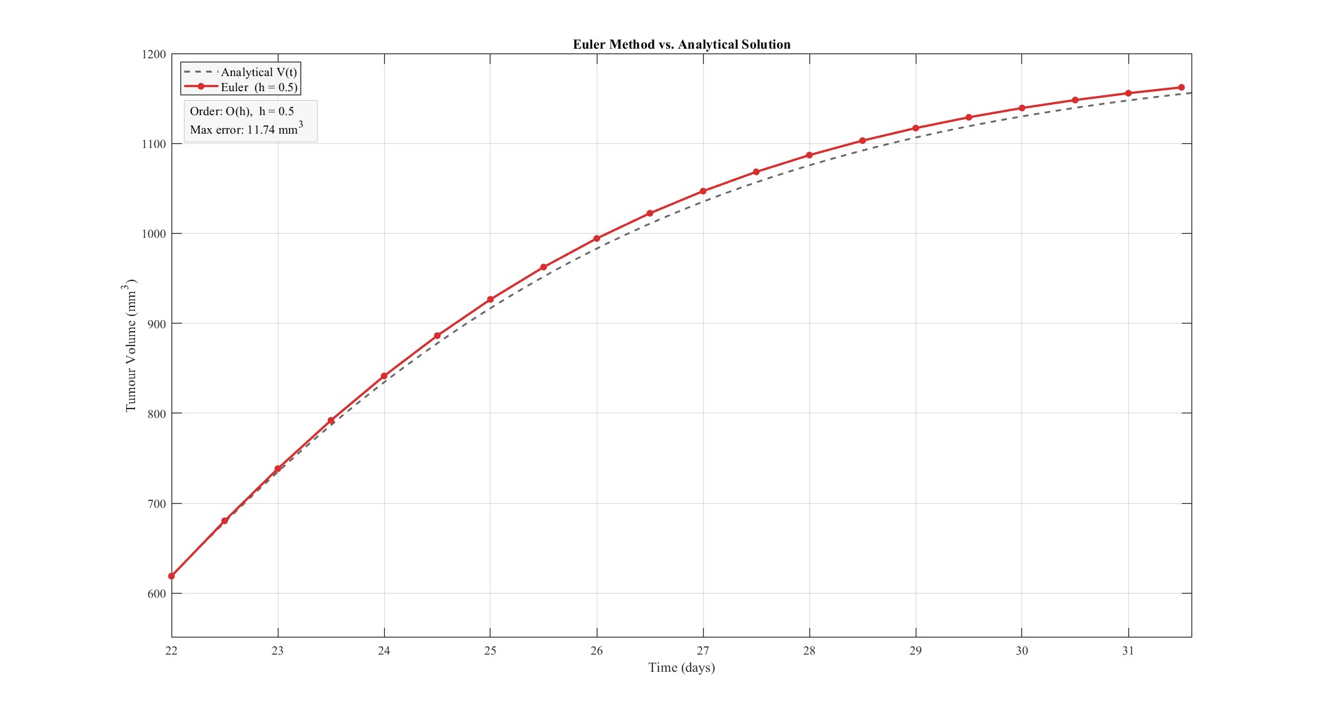
While the Gompertz equation has an analytical solution, biological models often become too complex (e.g., adding erratic drug dosing) to solve by hand. We must rely on numerical approximations.
The explicit Euler method computes the next volume based purely on the current tangent: $V_{n+1} = V_n + \Delta t \cdot f(t_n, V_n)$. Because it relies on a single slope, it is a first-order method $\mathcal{O}(h)$. In rapid tumour growth, it systematically overshoots the true curve.
Runge-Kutta 4th Order (RK4)
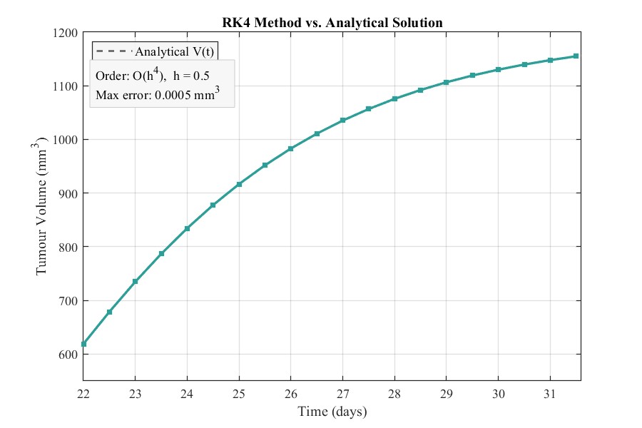
To reduce error without infinitesimally small time steps, we implement RK4. It computes four slopes ($k_1, k_2, k_3, k_4$) across the interval and takes a weighted average.
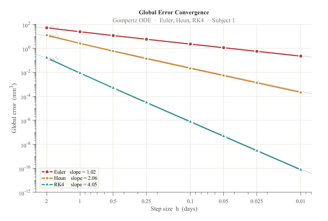
As a fourth-order method $\mathcal{O}(h^4)$, RK4 hugs the analytical truth flawlessly. Our log-log error analysis in MATLAB confirmed this exact order of convergence.
% 1. Define Model Parameters
a = 0.3;      % Intrinsic growth rate
K = 1200;     % Carrying capacity (mm^3)
V0 = 619;     % Initial volume (mm^3)
tspan = [22 32];
dt = 0.5;     % Step size

% Gompertz ODE Function
f = @(t, V) a * V * log(K / V);

% ------------------------------------------------
% 2. Explicit Euler Method (O(h))
tE = tspan(1):dt:tspan(2);
VE = zeros(size(tE));
VE(1) = V0;

for i = 1:(length(tE)-1)
    VE(i+1) = VE(i) + dt * f(tE(i), VE(i));
end

% ------------------------------------------------
% 3. Runge-Kutta 4th Order (O(h^4))
tR = tspan(1):dt:tspan(2);
VR = zeros(size(tR));
VR(1) = V0;

for i = 1:(length(tR)-1)
    k1 = f(tR(i), VR(i));
    k2 = f(tR(i) + dt/2, VR(i) + dt/2 * k1);
    k3 = f(tR(i) + dt/2, VR(i) + dt/2 * k2);
    k4 = f(tR(i) + dt, VR(i) + dt * k3);
    VR(i+1) = VR(i) + (dt/6) * (k1 + 2*k2 + 2*k3 + k4);
endHow fast does the error vanish?
A log-log plot of global error versus step size $h$ reveals the convergence order of each method. The slope of each line on this plot equals the theoretical order: Euler at $\mathcal{O}(h)$, Heun at $\mathcal{O}(h^2)$, and RK4 at $\mathcal{O}(h^4)$. Our MATLAB implementation confirms slopes of approximately 1, 2, and 4 respectively — validating that our solver implementations are correct.
RK4's fourth-order accuracy matters clinically: when modelling treatment response where small volume errors can misclassify whether a dose is above or below the tumour-static threshold $d^*$, the tighter error bounds of RK4 are essential.
Global Error Convergence — log-log · Euler, Heun, RK4
The number nobody measured.
Our supervisor asked a sharp question: how was $V_0$ obtained? The honest answer is that $V_0 = 619$ mm³ was never measured. It is the output of a three-stage chain, and each stage adds a layer of assumption.
Stage 1 — physical measurement. Tumours were sized with calipers, giving a largest diameter $L$ and a smallest diameter $w$. Volume was computed from the ellipsoid approximation used in the source study:
This already carries error. Calipers measure through skin, the ellipsoid assumption is geometric idealisation, and repeat measurements on the same tumour typically disagree by 10–20%.
Stage 2 — interpolation. Only five caliper readings exist for Subject ID=1 across the whole study. Day 22 is not one of them. Subramanian et al. fit a sigmoid through the five sparse points,
and read the model's initial condition off that fitted curve. So $V_0 = s(22) = 619$ mm³. It is an interpolated value, not an observation. The paper does not publish $A$, $k$ or $t_m$, which is precisely why our replicated sigmoid in Section V sits slightly off theirs.
Stage 3 — why it survives scrutiny anyway. Rather than defend the number, we quantify how much it matters. Because the solution is Gompertz, any error in the initial condition decays exponentially in log-volume:
Over the observation window $t - t_0 = 9.6$ days, the damping factor is $e^{-0.3 \times 9.6} = 0.056$. A 10% error in $V_0$ has shrunk to under 0.6% by day 31.6. The model forgets its initial condition at rate $a$ — so the weakest number in the parameter set is also the one the results depend on least.
Two further points close the question. First, $V_0$ has zero influence on the long-run equilibrium: as Section IX shows, the steady state depends only on $a$, $K$ and $d$. Second, the parameters $a = 0.3$ day⁻¹ and $K = 1200$ mm³ were obtained by the authors through nonlinear fitting with a TRBDF2 solver, so they carry their own fitting uncertainty — which we treat explicitly in the sensitivity analysis of Section XI.
What we would do with more data. The mathematically cleanest route is to stop treating $V_0$ as given and estimate it jointly with $a$ and $K$ by nonlinear least squares on the five raw caliper points, then report a confidence interval and check whether 619 falls inside it. With five points and three parameters this is possible but poorly conditioned, which is why we report it as the correct method rather than claim it as a result.
What a dose actually does.
The published model describes a tumour left alone. We extend it with a proportional kill term, giving the treated Gompertz equation:
The term $-dV$ encodes the log-kill hypothesis: a therapy removes a fixed fraction of tumour cells per unit time, so the absolute number killed scales with how much tumour is present. The parameter $d$ has units of day⁻¹ — the same units as $a$. It is an effective kill rate, not a drug mass.
Step 1 — the model collapses. Factor the right-hand side:
= aV [ ln(K/V) − ln(ed/a) ]
= aV ln( K e−d/a / V )
Defining the treated ceiling $K' = Ke^{-d/a}$, the treated model is exactly the original Gompertz model with $K$ replaced by $K'$ and $a$ unchanged. This is not an approximation. It is an identity.
A constant proportional therapy is mathematically indistinguishable from a tumour with a lower carrying capacity. We state this plainly rather than hide it: as a standalone modification, $-dV$ is a reparameterisation, not new dynamics. Its value is that it gives us a closed-form dose axis — and, as Section X shows, a linear system.
Step 2 — equilibria. Setting $dV/dt = 0$ with $V > 0$:
and $V = 0$ is a second equilibrium, since $V\ln(K/V) \to 0$ as $V \to 0^+$.
Step 3 — stability. Differentiating $f(V) = aV\ln(K/V) - dV$:
f′(V*) = a (d/a) − a − d = −a
$f'(V^*) = -a$ for every value of $d$. The dose decides where the tumour settles; it has no effect whatsoever on how fast it gets there. The system relaxes with time constant $\tau = 1/a = 3.33$ days regardless of how hard you treat.
As $V \to 0^+$ we get $f'(V) \to +\infty$, so $V = 0$ is unstable. The tumour is repelled from zero. Therefore $V^* = Ke^{-d/a}$ is globally asymptotically stable on $V > 0$.
Step 4 — the analytical solution. Because the model is Gompertz in disguise, the closed form carries over directly:
Setting $d = 0$ gives $K' = K$ and recovers the untreated solution of Section IV exactly — our reduction check.
Step 5 — the tumour-static dose. Imposing $dV/dt = 0$ at $t = t_0$ gives $aV_0\ln(K/V_0) - dV_0 = 0$, hence
Substituting back: $K'(d^*) = 1200\,e^{-0.1986/0.3} = 618.9 \approx V_0$. So $d^*$ is exactly the dose at which the tumour's equilibrium equals its starting volume.
We previously called $d^*$ a critical dose. That name is wrong and we have changed it. $d^*$ is a tumour-static dose — the boundary between growth and regression, not between survival and cure. Nothing curative happens at $d^*$.
| Regime | Behaviour from $V_0$ | Long-run volume |
|---|---|---|
| d < d* | Tumour grows | $K' > V_0$ |
| d = d* | Tumour held constant | $K' = V_0 = 619$ mm³ |
| d > d* | Tumour regresses | $K' < V_0$ |
Step 6 — does the model predict cure? No, and this is the most important thing our extension reveals. Since $V^* = Ke^{-d/a} > 0$ for every finite $d$, the tumour never reaches zero.
Near $V = 0$ the per-capita growth rate $a\ln(K/V)$ diverges to infinity, while the per-capita kill rate stays fixed at $d$. Growth always eventually wins. Eradication is impossible for any finite constant dose — not because the dose is too small, but because the structure of the therapy term is wrong for the job.
We can make this quantitative. If we define a practical detection threshold $V_{\text{det}}$, the dose needed to push the equilibrium below it is $d_{\text{det}} = a\ln(K/V_{\text{det}})$. For $V_{\text{det}} = 1$ mm³:
That is more than ten times $d^*$. The model therefore delivers a defensible clinical statement: under sustained proportional therapy, holding a tumour in check is cheap, and driving it to undetectability is extraordinarily expensive.
A tumour is a first-order system.
The Gompertz equation is nonlinear, which is why it needs numerical solvers. But one substitution removes the nonlinearity entirely. Let $u = \ln V$. Then $u' = V'/V$, and:
= a ln(K/V) − d
= a (ln K − u) − d
In log-volume, the treated Gompertz tumour is a first-order linear time-invariant system driven by the dose. Every tool from this course applies directly: integrating factors (M1), Laplace transforms (M3), eigenvalue stability (M4), and Fourier series for periodic dosing (M6).
The engineering reading. Taking Laplace transforms with $d(t)$ as the input and $u(t)$ as the output, the transfer function is
| System property | Value | Biological meaning |
|---|---|---|
| Pole | $s = -a = -0.3$ | Tumour is stable and self-limiting |
| Time constant $\tau$ | $1/a = 3.33$ days | How fast the tumour responds to a dose change |
| Settling time ($5\tau$) | $\approx 16.7$ days | Time to reach the new plateau |
| DC gain | $-1/a = -3.33$ | Each unit of dose lowers $\ln V^*$ by $1/a$ |
Steady state gives $u_{ss} = \ln K - d/a$, so $V^* = Ke^{-d/a}$ — the same equilibrium derived in Section IX, now recovered as the DC response of a first-order filter. The two derivations agree, which is our internal consistency check.
Why this matters for scheduling. Because the system is linear in $u$, a time-varying dose $d(t)$ with mean $\bar{d}$ produces a steady-state mean log-volume of $\ln K - \bar{d}/a$, regardless of how the dose is distributed in time. The schedule does not move the average; only the total dose does.
For a periodic dosing schedule of frequency $\omega$, the $n$-th Fourier harmonic of $d(t)$ is attenuated in $u$ by $1/\sqrt{a^2 + \omega_n^2}$. Dosing fast compared to $a$ ($\omega \gg 0.3$) gives a curve nearly identical to continuous infusion; dosing slowly ($\omega \lesssim 0.3$) produces large volume oscillations between cycles. The tumour smooths the treatment schedule exactly as an RC circuit smooths a square wave.
This reframing is what makes our extension more than an extra parameter. The untreated Gompertz model has no input, no pole and no gain — there is nothing to control. Adding $d$ turns a descriptive growth curve into a plant with a control input, and that is the object an engineer knows how to reason about.
Turn the dial, watch the ceiling fall.
With $a$, $K$ and $V_0$ held fixed, sweeping $d$ traces the entire behaviour of the treated model. Move the slider: the left panel shows the trajectory $V(t)$ against the untreated baseline, the right panel shows where the current dose sits on the dose–equilibrium curve $V^* = Ke^{-d/a}$.
Trajectory — treated vs untreated · x: time (days) · y: volume (mm³)
Dose–equilibrium law · x: dose $d$ (day⁻¹) · y: $V^*$ (mm³, log scale)
Read the right-hand curve carefully. On a logarithmic axis, $V^* = Ke^{-d/a}$ is a straight line with slope $-1/a$. It descends without limit but never touches zero — the graphical statement of Result 3. Reaching 1 mm³ requires $d = 2.13$ day⁻¹.
The dose sweep we report. Eight values, chosen to bracket $d^*$:
| $d$ (day⁻¹) | Relative to $d^*$ | $K' = 1200e^{-d/0.3}$ | Outcome |
|---|---|---|---|
| 0.000 | baseline | 1200.0 mm³ | Untreated growth to $K$ |
| 0.050 | far below | 1015.8 mm³ | Growth, slightly slowed |
| 0.100 | below | 859.8 mm³ | Growth, clearly suppressed |
| 0.1986 | equal to $d^*$ | 618.9 mm³ | Stasis — flat at $V_0$ |
| 0.250 | above | 521.5 mm³ | Regression to 522 mm³ |
| 0.400 | well above | 316.3 mm³ | Rapid regression |
| 0.600 | far above | 162.4 mm³ | Steep decline, 162 mm³ residual |
| 2.130 | $= d_{\text{det}}$ | 1.0 mm³ | Below detection — still not zero |
Sensitivity to the other parameters. Rather than sweeping blindly, we compute normalised sensitivity indices of the equilibrium $V^* = Ke^{-d/a}$, defined as $S_x = \frac{x}{V^*}\frac{\partial V^*}{\partial x}$:
| Parameter | Index $S_x$ | Value at $d = d^*$ | Interpretation |
|---|---|---|---|
| $K$ | $+1$ | $+1.000$ | Equilibrium scales one-for-one with carrying capacity |
| $a$ | $+d/a$ | $+0.662$ | Faster-growing tumours resist a fixed dose |
| $d$ | $-d/a$ | $-0.662$ | Equal and opposite to $a$ — only the ratio $d/a$ matters |
| $V_0$ | $0$ | $0.000$ | No effect on equilibrium; transient only |
$K$ dominates, so uncertainty in the carrying capacity propagates directly into every prediction. $a$ and $d$ have exactly equal and opposite influence, meaning the model has one effective control variable, the ratio $d/a$, not two. And $S_{V_0} = 0$ closes the loop on Section VIII: the parameter our supervisor questioned is the only one with no influence at all on the long-run result.
We therefore sweep $a$ and $K$ at $\pm 20\%$ and $V_0$ at $\pm 10\%$, and report the resulting envelope rather than a single curve.
What this model cannot do.
A model is only as useful as the honesty of its boundaries. We list ours.
| Limitation | Consequence |
|---|---|
| Constant $d$ reduces to lower $K$ | Our extension adds no new dynamics until $d$ varies in time |
| No eradication for finite $d$ | The model cannot describe cure, only suppression |
| No pharmacokinetics | $d$ is an effective rate, not a prescribable drug dose |
| No resistance or heterogeneity | Relapse under sustained therapy cannot be reproduced |
| Single compartment, no metastasis | Spread is outside the model entirely |
| Parameters from one murine subject | No claim of generality across subjects or species |
| No treated experimental data | The treatment model is validated numerically, not empirically |
| Mid-phase overestimation (Section V) | The Gompertz form itself misfits days 25–28 |
Validation status. Our untreated model is validated against published data. Our treated model is validated only against its own analytical solution — RK4 reproduces $V(t) = K'\exp(\ln(V_0/K')e^{-a(t-t_0)})$ to machine precision. Proper validation would require a treated experimental arm, fitting $d$ to it, and testing whether the observed plateau matches $Ke^{-d/a}$. We do not have that data and do not claim otherwise.
Why the contribution matters
| Question | Untreated Gompertz | Our extension |
|---|---|---|
| Where does the tumour settle? | Always $K$ | $Ke^{-d/a}$ — a function of dose |
| What dose holds it steady? | Unanswerable | $d^* = a\ln(K/V_0) = 0.1986$ |
| Can therapy cure it? | Unanswerable | Not for finite constant $d$ — proved |
| How fast does it respond? | — | $\tau = 1/a = 3.33$ days, dose-independent |
| Does the schedule matter? | — | Only through the mean dose; schedule sets the ripple |
| What kind of system is it? | Nonlinear growth curve | First-order LTI plant in $\ln V$ |
Future work
We separate what we did from what we would do next. Our contribution is the constant-dose extension, its equilibrium and stability analysis, the log-linearisation, and the sensitivity study above. Future work falls into three tractable steps:
1. Periodic dosing $d(t)$. A square-wave schedule with period $T$ and on-fraction $\varphi$. This is not reducible to a constant $K'$, requires numerical integration, and is solvable analytically by Fourier series through the low-pass result of Section X. This is the natural next step and the one we recommend.
2. A saturating kill term. Replacing $-dV$ with a term whose per-capita effect does not vanish near $V = 0$ would allow finite-time eradication, isolating structure rather than magnitude as the barrier to cure.
3. Resistance. Splitting $V$ into sensitive and resistant compartments gives a $2\times2$ system, phase-plane analysis, and the relapse behaviour a single compartment cannot produce.
We took a descriptive growth curve, gave it an input, proved where it settles and how fast, showed that it is a first-order linear system in log-volume, and established that constant proportional therapy can suppress a tumour indefinitely but can never eliminate it.
The project, hand-drawn.
Everything above condensed into a single illustrated panel: the biology, the equation, the simulation, and the reason any of it matters. It reads as five numbered stages, moving from cells competing for limited resources through to predictions that inform treatment planning.
Modelling Tumour Growth Using the Gompertz Model — Illustrated Summary

Reading the panel. Stage 1 establishes why growth has to saturate at all: cells multiply, but resources are finite. Stage 2 places that competition inside a living system. Stage 3 is the translation step, where biology becomes $dV/dt = aV\ln(K/V)$ and the sigmoid curve it generates, with the inflection point sitting at $V = K/e$. Stage 4 turns the predictions into use, and Stage 5 is the MATLAB work of Sections VI and VII, where the equation is actually solved.
The inflection point deserves a note. For the Gompertz model, growth is fastest at $V = K/e \approx 441$ mm³. Our observation window opens at $V_0 = 619$ mm³, which is already past that point — so every curve on this site sits on the decelerating branch of the illustration. The tumour was doing its fastest growing before the data begins.
Final Submission · Group 5
We
modelled you.
Oh, but we did.
Growth, treatment, equilibrium, stability — and the honest
admission that at $d = 0.60$ day⁻¹ you still have 162 mm³ left.